How to Use VLOOKUP in Excel

VLOOKUP is an Excel function. VLOOKUP is a database function in short; we can say that it works with database tables. In simple terms VLOOKUP Excel function helps us to find information about selected cells from another Excel document. So it is an amazing function and time saving. Here is an example to understand the function of VLOOKUP. For example you want to find something about apple then VLOOKUP look for this piece of information (i.e. apple) or also find the related information like price of apple. Just one query can save your lots of time. Let’s have a look below to solutions on how to use VLOOKUP in Excel.

• 1: How to Do VLOOKUP from Another Worksheet
• 2: How to VLOOKUP from A Different Workbook
• 3: How to Use A Named Range or Table in VLOOKUP Formulas
• 4: Using Wildcard Characters in VLOOKUP Formula

1: How to Do VLOOKUP from Another Worksheet

First I am going to explain how to use VLOOKUP in Excel so that you can easily understand how to do VLOOKUP from another worksheet.

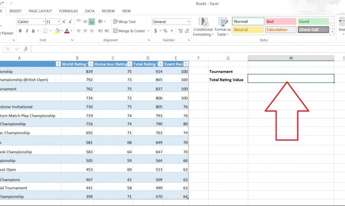
Step 1: First you need to choose the cell where you want to calculate VLOOKUP formula.

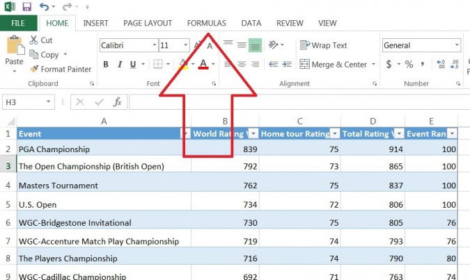
Step 2: In second step you need to choose formula from the top bar.

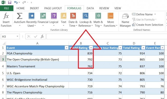
Step 3: Now you need to choose Lookup & Reference.

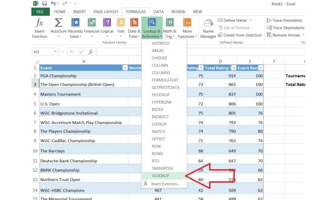
Step 4: Here you will find a dropdown menu, just choose VLOOKUP from there.

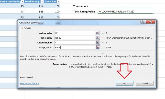
Step 5: Now you will find a table as you can see in the picture below

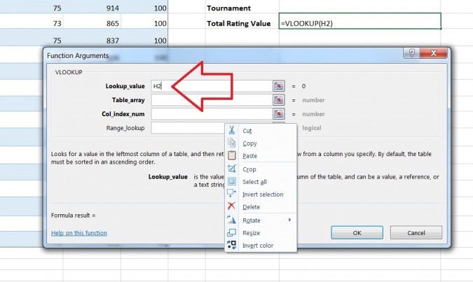
Step 6: If you have found a table like an image above, first you need to specify a cell and you need to enter the value whose data you are looking for. We are going to choose H2, because our lookup value is H2.

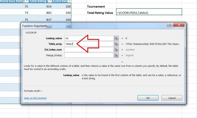
Step 7: After choosing LOOKUP value, now you need to specify the table array. We are going to choose entire table as we are calculating total rating for PGA Championship you can see in the picture.

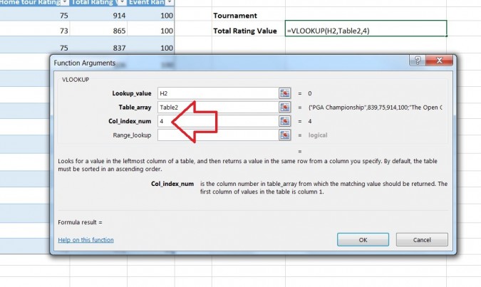
Step 8: Now you need to specify the column number, as we are calculating total rating Column D so we are going to enter column 4.

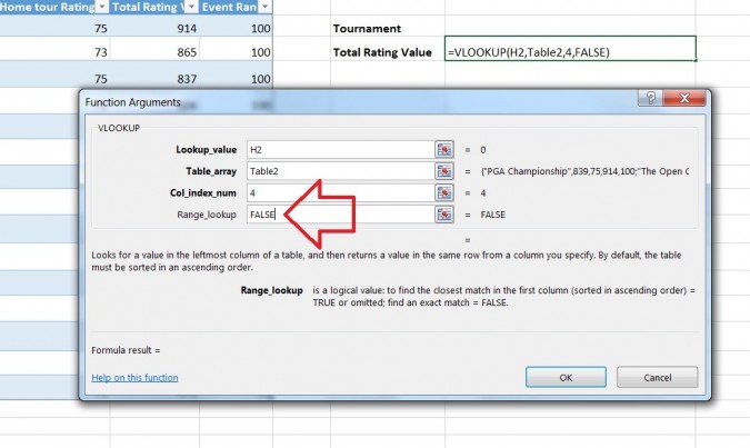
Step 9: Now you need to enter range in the range lookup box. If you will enter TRUE, LOOKUP will show the results with approximate match. But if you choose FALSE, LOOKUP will find an exact match result s we are going to choose FALSE.

Step 10: Now you need to choose the OK button to proceed.

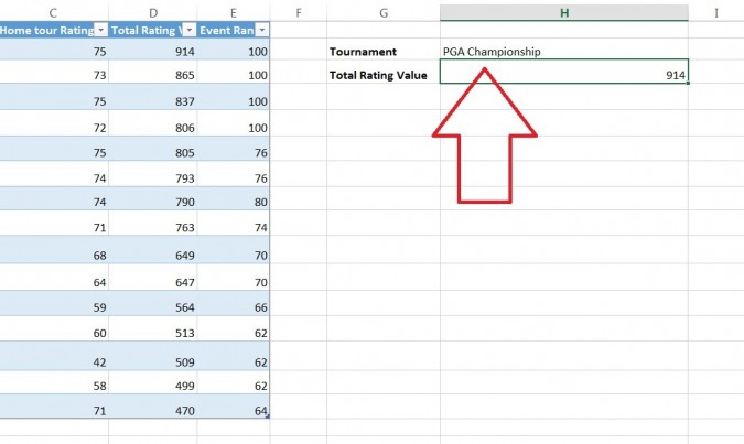
Step 11: As we were finding total rating of PGA Championship so we type PGA Championship in H2. You can see VLOOUP auto finds the total rating in H3 as 914.

Well, if you want to find data from different workbooks then this is quite simple as compared to find data from same sheet.

Let’s have a look to this formula:

=VLOOKUP(B5,Sheet2!$B$5:$C$104,2,0)

If you type this query, VLOOKUP finds correct building for each employee on sheet 2 into the table on sheet 1.

Let’s have a look below to this picture.

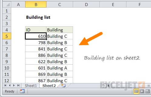
On sheet 1 we are going to find the building location for each team member by using this formula.

=VLOOKUP(B5,Sheet2!$B$5:$C$104,2,0)

As you can see for Lookup value we have used column B, the employee id. And for the table array we have used B54:$C$104 that includes a sheet name too.

Sheet2!$B$5:$C$104 // includes sheet name

This is the simple formula for finding data from another worksheet. When you enter the sheet name you simply tell VLOOKUP which sheet to use for table LOOKUP range.

Finally, column number is 2 because building appears in the second column. And VLOOKUP is set to exact match by including zero to show exact results.

2: How to VLOOKUP from A Different Workbook

We have already introduced how to do VLOOKUP in Excel now let’s have a look to a formula to use VLOOKUP for external Workbook.

=VLOOKUP(B5,'[product data.xlsx]Sheet1'!$B$5:$E$13,4,0)

This formula is almost same like we use VLOOKUP from another sheet. The only difference is of syntax.

Let’s have a look to syntax for using external workbook:

'[workbook]sheet'!range

Here in the place of workbook you can replace the name of external workbook (i.e. file.xlsx)

Sheet is the name of sheet that containing ranges (i.e. Sheet1 or Sheet2)

Last one is the range that represents actual range for table array (i.e. A1:C100)

Use this formula and enjoy VLOOKUP functionality for external workbooks too.

3: How to Use A Named Range or Table in VLOOKUP Formulas

After getting knowledge to how to do a VLOOKUP now let’s have a look to a functionality of named range. On the off chance that somebody needs to call me, they will call my name. Isn't that so? Thus, in Excel, you can give a name to a cell. For example, B1 or B1:B10, you can just utilize the name that you allotted to it.

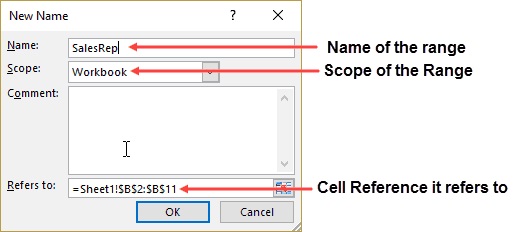
First you need to choose the range for which you need to make a Named Range in Excel and then go to Formulas > Define Name.

A dialogue box will appear, just type the name that you want to assign to that cell and press OK.

4: Using Wildcard Characters in VLOOKUP Formula

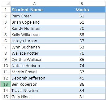
Want to make VLOOKUP more powerful? Wildcard helps to find a value using a partial match. Let’s have a look to an example below to understand wildcard characters.

For example, you want to find a student marks with their first name. Then you will use asterisk which is a wildcard character with first name.

Types of wildcard characters:

• Asterisk (*): You can use “Ba*” to match the text “Banana”.
• Question Mark (?): you can use E?cel to find for the text “Excel”
• Tilde (~): This character will help you to nullify the effect of above character. You can use it like that "PD~*.

Summary

The short conclusion of this article is that first we introduced different solutions on how to VLOOKUP in Excel, how to use VLOOKUP to find data from another sheet as well as how to find wild characters using VLOOKUP. We have also introduced a great solution to recover a forgotten password of Excel. Hope you like this article, if you like then share it with others. And make sure to subscribe our newsletter for more updates.

By the way, if you forgot your open password in Excel, then we will recommend SmartKey Excel Password Recovery to you. This tool is just amazing to recover lost passwords for Excel worksheet, tested by experts and 100% secure.

Download SmartKey Excel Password Recovery:

comments powered by Disqus